Capacity of a Discrete Channel
A system whereby a sequence of choices from a finite set of elementary symbols can be transmitted from one point to another. Each of the symbols is assumed to have a certain duration in time seconds (not necessarily the same for different ).
Referenced by (1 direct, 3 transitive)
Direct references:
Transitive (depth 1):
The capacity of a discrete channel is given by
where is the number of allowed @signals of duration
Referenced by (3 direct)
Direct references:
Given an information source where all symbols are of the same time duration, and each symbol represents bits of information (because it is chosen freely among symbols), and the channel can transmit symbols per second then the capacity of the channel is defined to be bits per second.
In the more general case we have to deal with symbols of various lengths that take different amounts of time to transmit, and so capacity measures not the number of symbols transmitted per second but the amount of information transmitted per second, retaining bits per second as its unit.
If represents the number of sequences of duration then
This number is equal to the sum of the numbers of sequences ending in This is a recursive definition - if the last symbol is and then we have time remaining for the previous symbols in the sequence, and we repeat the same question on that remainder.
A "well-known result" in finite differences tells us that
where is constant and is the largest real solution of the characteristic equation:
and therefore
Consider Morse code as used in telegraph. We have the following rules:
- A dot symbol consists of one time unit of line closure followed by one time unit of line open.
- A dash symbol consists of three time units of line closure followed by one time unit of line open.
- A letter space symbol consists of three time units of line open.
- A word space symbol consists of six time units of line open.
We're never allowed to send two space symbols in a row, because two sequential letter space symbols are indistinguishable from a word space symbol.
Now, our possible terminating states are
| Symbol | Composition | Duration (time units) |
|---|---|---|
| Dot | 1 unit closed + 1 unit open | 2 |
| Dash | 3 units closed + 1 unit open | 4 |
| Letter space preceded by dot | 1 unit closed + 4 units open | 5 |
| Letter space preceded by dash | 3 units closed + 4 units open | 7 |
| Word space preceded by dot | 1 unit closed + 7 units open | 8 |
| Word space preceded by dash | 3 units closed + 7 units open | 10 |
Note that we had to consider the last two symbols in the case of the last symbol being a space in order to deal with our "no sequential spaces" constraint.
Now we have
So, our characteristic equation is
With a substitution of we get
and the largest positive root of this equation, found numerically, is about and so
Note that in this Morse telegraphy system, we have two states that the channel can be in, based on what the previous symbol transmitted was.
- If the previous symbol transmitted was a space, we're in state and the next symbol can only be a dot or a dash, and the state will change.
- If the previous symbol transmitted was not a space, we're in state and the next symbol can be anything, and the state may or may not change depending on what the next symbol is.
We can think of these states being the @nodes of a @directed-graph with the transitions between them being the @edges. A generalization of this is given in the theorem below.
Let be the duration of the -th symbol which is allowable in state and leads to state Then the channel-capacity is equal to where is the largest real root of the @determinantal-equation
where is the @Kronecker-delta.
For example, for our Morse telegraphy example, we have
Expanding the @determinant on the LHS gives the characteristic equation above.
Information and Entropy in a Discrete Channel
Given a real number and an outcome of a discrete random variable with probability mass function the self-information of is defined as the negative log probability
Referenced by (5 direct, 29 transitive)
Direct references:
Transitive (depth 1):
- Cross-Entropy
- doubly-stochastic-maps-increase-entropy-intuition
- Entropy Rate
- Gibbs' Inequality
- Chain rule for joint entropy
- joint-entropy-is-less-than-or-equal-to-entropy-of-parts
- KL Divergence
- Noiseless channel transmitting discrete symbols
- note-25
- note-8
- proof-of-concavity-of-entropy
- proof-of-doubly-stochastic-maps-increase-entropy
- proof-of-joint-entropy-is-less-than-or-equal-to-entropy-of-parts
- proof-of-uniform-distribution-maximizes-entropy
- remark-14
- theorem-12
- Uniform distribution maximizes entropy
- Weak Asymptotic Equipartition Property
Transitive (depth 2):
- Model Training
- Strong Asymptotic Equipartition Property (Shannon--McMillan--Breiman)
- proof-of-nonnegativity-of-conditional-mutual-information
- proof-of-nonnegativity-of-conditional-relative-entropy
- proof-of-nonnegativity-of-mutual-information
- proof-of-nonnegativity-of-relative-entropy
- proof-of-chain-rule-for-entropy
- proof-of-mutual-information-and-entropy
- proof-of-theorem-54
- remark-32
- concavity-of-entropy-intuition
We can view self-information as an alternative casting of probability, like how odds are, with some desirable properties:
- An event with probability provides no information - we knew it was going to happen so it happening tells us nothing new.
- The less probable an event is, the more surprisal it yields.
- self-information is @additive - if two individual events are measured separately, the total amount of information is the sum of the self-informations of the individual events.
The function given above is the unique function of probability (up to a multiplicative scaling factor) that satisfies these three properties.
In a related vein we can develop a function that asks how much choice is involved in the selection of an event, or equivalently, how much uncertainty there is in the outcome. If are the probabilities of events occurring, we want a measure that has the following properties:
- should be continuous in the That is, a small change in a should result in a small change in
- If all the are equal, then should be a @monotonic @increasing function of With equally likely events there is more choice, or uncertainty, when there are more possible events.
- If a choice is broken down into two successive choices, the original should be the weighted sum of the individual values of For example, we should have that
Given a discrete random variable which may be any element within the set and is distributed according to the entropy is
We can choose different bases for the logarithm; throughout these notes a bare means giving the unit of @bits.
An alternative, equivalent definition is that entropy is the expected value of the self-information of a random variable:
The unit for entropy is bits per symbol.
Referenced by (21 direct, 11 transitive)
Direct references:
- Discrete Entropy
- theorem-12
- remark-14
- theorem-16
- note-25
- Chain rule for joint entropy
- Cross-Entropy
- KL Divergence
- Gibbs' Inequality
- Uniform distribution maximizes entropy
- proof-of-uniform-distribution-maximizes-entropy
- joint-entropy-is-less-than-or-equal-to-entropy-of-parts
- proof-of-joint-entropy-is-less-than-or-equal-to-entropy-of-parts
- proof-of-doubly-stochastic-maps-increase-entropy
- doubly-stochastic-maps-increase-entropy-intuition
- proof-of-concavity-of-entropy
- Entropy of a Discrete Information Source
- Entropy Rate
- Weak Asymptotic Equipartition Property
- Noiseless channel transmitting discrete symbols
- note-8
Transitive (depth 1):
- Model Training
- Strong Asymptotic Equipartition Property (Shannon--McMillan--Breiman)
- proof-of-nonnegativity-of-conditional-mutual-information
- proof-of-nonnegativity-of-conditional-relative-entropy
- proof-of-nonnegativity-of-mutual-information
- proof-of-nonnegativity-of-relative-entropy
- proof-of-chain-rule-for-entropy
- proof-of-mutual-information-and-entropy
- proof-of-theorem-54
- remark-32
- concavity-of-entropy-intuition
Real numbers are commensurable if there exists a common measure such that each is an integer multiple of it: Equivalently, all pairwise ratios are rational: for all (with ).
Referenced by (1 direct)
Direct references:
The only satisfying the three required properties above is the entropy function defined above, up to multiplication by a constant.
Assume we have a function that satisfies the three properties listed above, such that
Then, by property (3) above, we can decompose a choice from equally likely possibilities into a sequence of choices each from equally likely possibilities. For example, if we have equally likely possibilities, the probability of any given event is . If we instead we have a series of choices each with probability, we end up with as the probability of any specific sequence of events. So, we have that
Now, with arbitrarily large we can also have such that by the same logic, and we can pick such that
Now, we can take the logarithm of each term to get
and dividing by gives
and because is arbitrarily large,
where is arbitrarily small.
By property (2) of (it is a @monotonically-increasing function of ,)
Then, dividing by gives
Now, by the @triangle-inequality, we have that
Since can be arbitrarily small, we have that with so that property (2) holds. Now we know what is, and thus what is when we have equal probabilities for all events.
Now let's say that we have a choice from possible events with commensurable probabilities We can break down a choice from possibilities into a choice from possibilities with probabilities and then, if the th possibility was chosen, choices of equal probability We do this because above, we found how to find when all events are equally likely, and property (3) of our desired function lets us break down our overall choice from possibilities. This gives us
Then,
If the are incommensurable, we can approximate them as closely as we'd like with rationals, since The rationals are dense in the reals.. By the first property we assumed for it is continuous in the and so its value at the incommensurable equals its limit as we approach via the rationals, and so our expression holds in general. is left to us to pick, picking it is equivalent to picking a base for the logarithm.
The entropy of a random variable quantifies the average level of uncertainty or information associated with the variable's possible outcomes. It measures the expected amount of information needed to describe the state of the variable, considering the distribution of probabilities across all potential states.
When we decrease the probability of an element occurring, its self-information increases only logarithmically, while its weight in the entropy sum decreases linearly.
The demo below makes these quantities concrete. It uses a discrete alphabet of symbols whose probabilities follow a Zipfian distribution,
where the skew controls how unevenly probability mass is spread across symbols. At every symbol is equally likely (the uniform distribution), so entropy is maximal at As grows the distribution concentrates on the first few symbols, the rare symbols carry ever more self-information, and the entropy falls toward The bar chart shows the probability of each symbol alongside its self-information; the second chart traces the entropy as sweeps from uniform to highly skewed.
Examples to cover: [https://claude.ai/chat/0702d3b2-a181-4b5b-a572-e5464d9d24d5]
Example: Coin Flip
For a fair coin flip, and Then, and
Let's say we have an unfair coin and Then
and for entropy of we get
Example: Six-Sided Die
For a fair six-sided die, and for all Then, and
Let's say we have an unfair die and and for Then
and for entropy of we get
Some Theorems on Entropy
When a random variable is uniformly distributed over an alphabet of elements, the self-information of any given element equals the entropy of the random variable and is
We use the Logarithm Change of Base here.
iff all the but one are zero, this one having the value of one.
Suppose Then, Note that because we have and (with the convention since ). Assume for contradiction that more than one is non-zero. Then, because each non-zero is in and therefore its and the sum of these terms is therefore non-zero, a contradiction. Now, since all probabilities are required to sum to 1, it can't be the case that all probabilities are zero, which means that exactly one probability must be non-zero and that probability must be
Joint and Conditional Entropy
The joint entropy of a pair of @discrete random variables with a joint distribution is defined as
which can also be expressed as
Referenced by (2 direct, 3 transitive)
Direct references:
Let and be random variables, not necessarily independent. The probability that takes the value when takes the value (for any specific ) is called the conditional probability and is given by:
(Note that is the joint probability of )
We define the conditional entropy of given as the average of the entropy of for each value of weighted according to the probability of getting that particular That is,
Referenced by (1 direct)
Direct references:
We can obtain the above formula for conditional entropy as follows. First, if then our entropy for is
Now, summing across gives:
The entropy (joint entropy) of the joint event is the entropy of plus the entropy of when is known, that is,
Note that
The first term on the RHS is just The second is
Altogether, we have that or
Referenced by (1 direct)
Direct references:
Referenced by (3 direct)
Relative Entropy and Mutual Information
Given two discrete probability distributions, and that share a support cross-entropy measures the average number of bits needed to represent an event drawn from when the coding scheme is optimized for an estimated distribution rather than the true distribution Its formula is very similar to that of entropy, except surprisal is calculated using while expectation uses :
We can write it in expectation form as
where is expectation under
Referenced by (5 direct, 6 transitive)
Direct references:
Note that when cross-entropy equals entropy. The symbol is overloaded: with distributions as arguments means cross-entropy, while with random variables as arguments means joint entropy.
For discrete probability distributions, and on a common alphabet the relative entropy from to is defined to be
which is just cross-entropy minus entropy:
Note that we don't always use the subscript where it's obvious from the context.
We can also write it as
which makes it clear that it's the expected inefficiency in an encoding optimized for rather than
Referenced by (1 direct)
Direct references:
kl divergence tells us how different an approximating distribution is from a true probability distribution It's not a true distance metric - it's asymmetric, but it does behave like distance in that it gets smaller as gets more like and is zero when It is a sort of directed distance.
Another way to think about it is as a measure of how inefficient a coding scheme optimized for is when the actual distribution is If says some event is rare, and so we use a longer symbol for it (more bits), but the event actually occurs frequently, we'll waste bits representing the event when we could have used a shorter symbol for it.
Consider two random variables and with joint probability mass function and marginal probability mass functions and The mutual information is the relative-entropy between the joint distribution and the product distribution :
Referenced by (1 direct)
Direct references:
Relationship Between Entropy and Mutual Information
We'll prove (c) first:
Now, from Chain rule for joint entropy we prove (a) and (b) with
and
(d) is trivial from symmetry of and
To prove (e) we use our result from (a):
Referenced by (1 direct)
Direct references:
Chain Rules
Let be drawn according to Then
From Chain rule for joint entropy, we have
Referenced by (1 direct)
Direct references:
The conditional mutual information of random variables and given is defined by
It is the uncertainty about after learning minus the uncertainty about after learning and .
Referenced by (1 direct)
Direct references:
From Mutual Information and Entropy we have
Then, from Chain Rule for Entropy and Chain Rule for Conditional Joint Entropy we have, simplifying,
Now, from our definition of conditional mutual information we get
For joint probability mass functions and the conditional relative entropy
is the @average of the relative-entropies between the conditional probability mass functions and averaged over the probability mass function More formally,
Referenced by (2 direct)
Inequalities
For discrete probability distributions and that share a support
with equality iff Equivalently, cross-entropy is never less than entropy: with equality iff
Because Log is Concave, by Jensen's Inequality we have that
Then, since we have that
Now, note that if and Conversely, suppose Since is strictly concave, it is not @affine, and Jensen's Inequality condition for equality gives us that Now, and since is a probability distribution, and therefore and
For any two random variables, with equality if and only if and are independent.
Using the definition of mutual information and Gibbs' Inequality, we have with equality if and only if i.e. and are independent.
with equality if and only if for all and such that
From the definition of conditional relative entropy we have
This is just the average of the relative-entropy over distributions over for each fixed For each is if and only if by Gibbs' Inequality, and positive otherwise.
with equality if and only if and are conditionally independent given
We have that
and for each fixed
.
By Gibbs' Inequality, the quantity for each fixed is non-negative, so the sum weighted by the probability of each is also non-negative.
For equality, the average is if and only if for each with
why by Gibbs' Inequality means
for all i.e. and are conditionally independent given
A random variable has the most entropy when the elements of its alphabet are all equally likely to occur.
We will use a @Lagrangian function of entropy to show this. Let
Then, for any we want
But, this means doesn't depend on and so is the same for each and therefore
It remains to show that this extreme of is a maximum. This follows from the facts that the domain is a convex, compact set and that the entropy function is strictly concave. TODO: more details on these.
Referenced by (1 direct)
Direct references:
The uncertainty of is never increased by knowledge of It will be decreased unless and are independent events, in which case it is not changed.
From Let and be discrete random... and Chain rule for joint entropy, we have
hence
Let and be discrete random variables with alphabets and and let be the probability of the joint occurrence of and
The entropy of the joint event (the joint entropy), is less than or equal to the sum of the individual entropies, i.e.
with equality iff and are independent, that is, iff
The entropy of the joint event is
This is just treating each possible pair of individual outcomes as its own outcome, i.e. we have possible outcomes. Writing and for the marginals (the argument names the distribution), we have
So,
Now, let's define a new random variable for convenience, We now have that
Now, by Jensen's Inequality, because Log is Concave, we have that Now,
Therefore and we have that and
Now, for the equality part. Suppose Then, and recalling that In Jensen's Inequality, equality holds only if our function is @affine or if is constant; since is @affine on no interval, must be constant, and since
Now, suppose Then and
so
Referenced by (1 direct)
Direct references:
Take a @doubly-stochastic matrix and probability vector let Then with equality iff is a @rearrangement of .
Note that by the definition of vector matrix multiplication. Now we'll define a couple of joint distributions:
Now we find the relative-entropy from to :
Now, addressing the first term on the RHS of the last line:
And the second term on the RHS of the last line:
So, we end up with Since by Gibbs' Inequality, we have which implies that which is what we wanted to show.
Now, the equivalence case. If is just a rearrangement of then obviously it has the same entropy as we can just re-index to recover Now assume Then, whenever Now, for each value appearing in or let
that is is the set of indices of where and similarly with and Now, consider row For any we have so i.e. every nonzero entry of row lies in a column of so the columns have the entire mass of row Similarly, for column for nonzero so and the rows contain all of column 's mass. Taking as the @indicator-vector of a set we have that
that is, rows in sum to over the columns while rows outside have no mass in the columns at all. Now we count the mass:
Therefore, for all so each appears equally often in and in and is therefore a rearrangement of
Averaging (well, replacing each probability with a convex combination of all the probabilities in a way that retains their summing to 1) the probabilities in can only bring them closer to each other (if it doesn't just rearrange them), which increases entropy.
Log Sum Inequality and Its Applications
For non-negative numbers, and
with equality if and only if
We use the conventions that if and all of which follow from @continuity.
We can assume without loss of generality, due to the -handling conventions specified above, that and Now, note that the function is @strictly convex, since for all positive Then, by Jensen's Inequality we have
as long as i.e. if the form a @discrete probability distribution.
If we let , i.e. is the @probability mass assigned to index then this condition is met. We can then pick and we get
Referenced by (2 direct)
For discrete probability distributions and that share a support
with equality if and only if
This restates Gibbs' Inequality, which the Log Sum Inequality proves more directly.
with equality if and only if Both and are probability mass functions, so (otherwise they wouldn't both sum to 1) and hence we have if and only if for all
TODO: Cover & Thomas Theorem 2.7.2.
is convex in the pair that is, if and are two pairs of probability mass functions, then
for all
First, note that the set of probability mass functions on is the set of probability vectors in where and thus is a convex set. takes a pair which is again convex, so is defined on a convex set.
Now we'll apply Log Sum Inequality to the one term with a fixed left-hand side of the inequality in the theorem, but we'll do some replacements to make it more obvious what's happening.
Let
Using those substitutions, with Log Sum Inequality, we have
Summing both sides of this over gives us
relative-entropy is a convex @surface over @pairs , with a flat-bottomed zero valley along , rising as and differ.
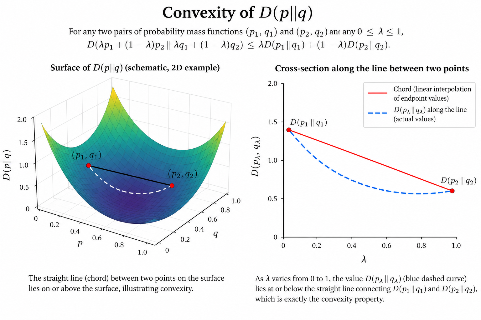 The image above was generated using GPT-5.6 Sol.
Another way to think of this is that mixing and , and and can't make the results more distinguishable than the weighted average distinguishabilities between and and and , i.e., mixing distributions tends to wash out distinctions.
Referenced by (1 direct)
Direct references:
is a concave function of
Let be the uniform distribution on outcomes. Then from the definition of @relative-entropy,
Then, from the definition of cross-entropy
So,
and by Convexity of Relative Entropy, entropy is a concave function.
The intuition is that mixing distributions can never decrease uncertaintity.
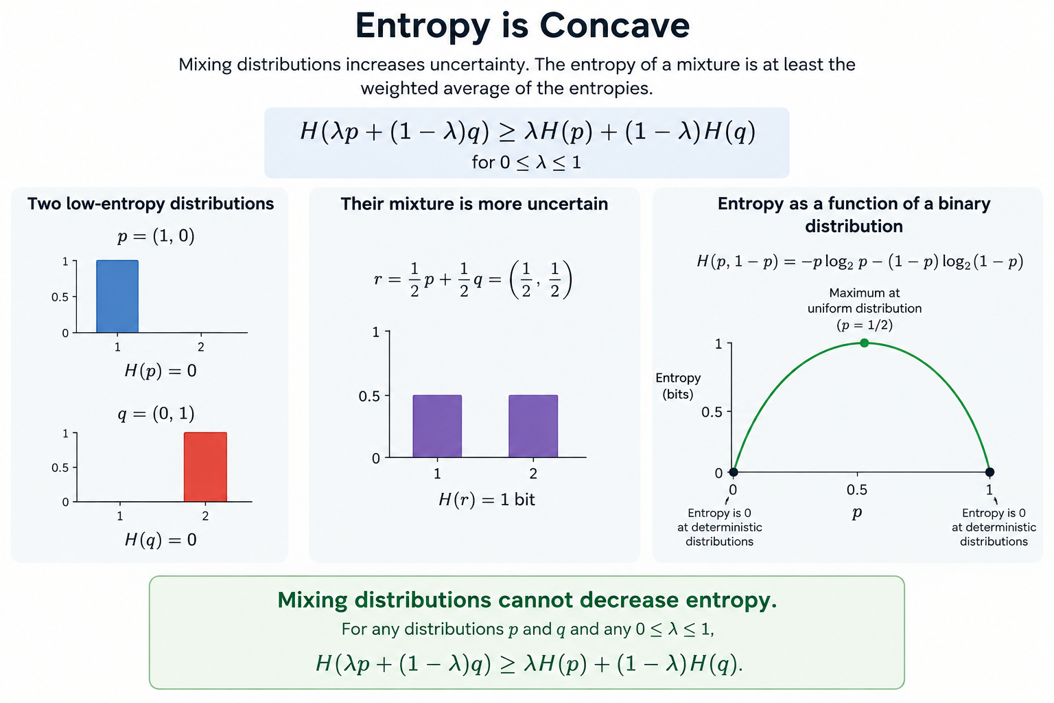 The image above was generated using GPT-5.6 Sol.
We already proved Uniform distribution maximizes entropy using Lagrangian multipliers, but the proof above shows it in another way. If then and since is constant in is maximized by .
TODO: Cover & Thomas Theorem 2.7.4.
Data-Processing Inequality
TODO: Cover & Thomas, Section 2.8.
Referenced by (4 direct)
TODO: Cover & Thomas Theorem 2.8.1.
TODO: Cover & Thomas, corollary to Theorem 2.8.1.
Sufficient Statistics
TODO: Cover & Thomas, Section 2.9.
TODO: Cover & Thomas, Section 2.9.
TODO: Cover & Thomas, Section 2.9.
Fano's Inequality
TODO: Cover & Thomas Theorem 2.10.1.
TODO: Cover & Thomas, Section 2.10.